The Cartoon Brain : Artificial Neural Networks

Introduction
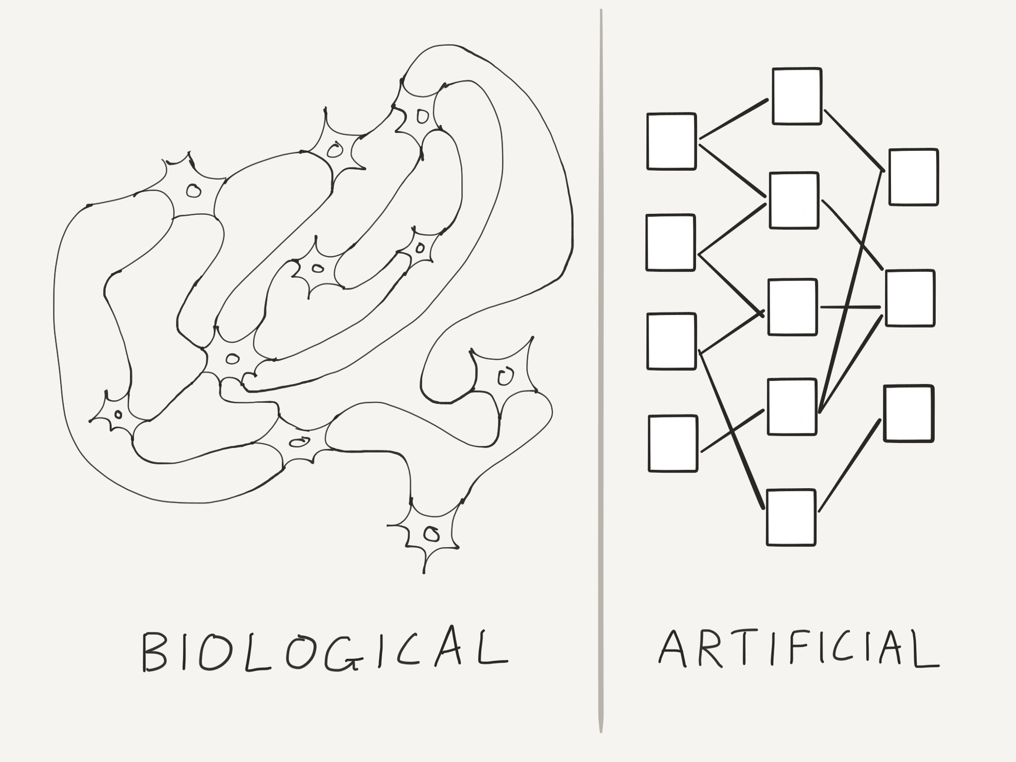
In this post we are going to talk about a learning technique that is, at least at the very minimum, based on the structure of a brain. The title of the blog post summarizes this approach.
While at first sight it might seem that with the terminology of neurons and neuronal weights we are modelling something like the brain, in reality, ANNs (Artificial Neural Networks) are really just complex non-linear (possibly linear) pattern recognition architectures.
A Few Points To Keep In Mind
Before we begin describing the architecture and how it works, it is important to keep in mind what the algorithms are really doing. It is very easy to get hung up into the machinery involved and lose sight of the big picture.
As noted at the start, these models are really cartoon models (oversimplifications) of the actual neurons in our brains. While these models work very well in many domains in practice, their applicability in understanding the neurophysiological basis of things is limited.
In this post we will use the term neuron to refer to an artifical neuron.
Let’s Begin

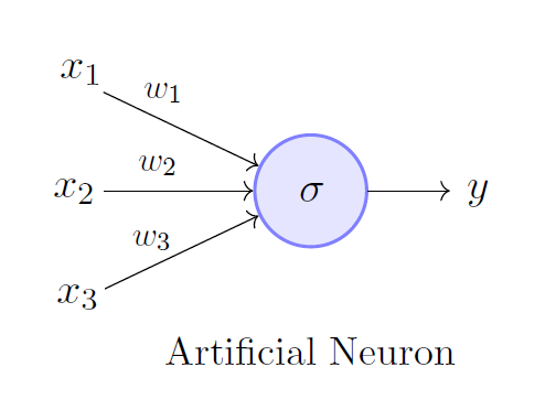
As the above image shows, in the most simple case, an artificial neuron has the basic computational structure of computing weighted sums of its inputs. In the above image, the output y is obtained from its inputs is obtained as follows:
\[y = \sum_{n=1}^3 (x_n * w_n) + b\]where the \(w_n\) , \(n = 1, 2, 3\) denote the weights and similary the \(x_n\) denote the inputs, the \(b\) parameter denotes the bias, or the offset. This simple computation is really the basis for most ANNs.
But notice how this computation is linear, in fact, the activation function \(f\) as it is so called, is the identity in this case, which means:
\[f(x) = x\]Using this we can write the computation in the above image as:
\[y = f(\sum_{n=1}^3 (x_n * w_n)) = \sum_{n=1}^3 (x_n * w_n) + b\]But linearity is boring, in fact, reality is non-linear and noisy. Here, we introduce non-linearities into the system by using other forms of \(f\) as opposed to the identity.
One non-linearity we have already seen is the sigmoid function in the post about logistic regression. There are other such functions used too, such as tanh, relu, etc. In fact, you can use a function of your own as long it is well behaved, code for differentiable.
The property of differentiability is going to come in handy later.
The logistic sigmoid is given by:
\[f(x) = \frac{1}{1 + e^{-x}}\]In our case, we can then write the computation of this neuron as:
\[y = f(\sum_{n=1}^3 (x_n * w_n)) = \frac{1}{1 + e^{\sum_{n=1}^3 (x_n * w_n) + b}}\]Multiple Neurons
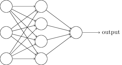
Now that we’ve seen the computation for a single neuron, you might think that the computational power of such a system is limited and indeed this is the case. However, we can easily this to multiple neurons, such as shown in the below image:

The first layer that you see is just the inputs, while the actual neurons are in the first hidden layer, where each neuron performs the computation defined by \(y\) just above, and the final layer is the output layer.
In this image, the input layer has three inputs, let us call them \(x_i, i = 1, 2, 3\). The hidden layer has four neurons, let us call them \(n_i, i = 1, 2, 3, 4\). The output is just one neuron, let us call it \(o\).
Forward Pass
Thus we can describe the computation of each \(n_i\) as shown below:
\[n_i = f(\sum_{k=1}^3 (x_k * w_{ik})) = \frac{1}{1 + e^{\sum_{k=1}^3 (x_k * w_{ik}) + b_i)}}\]where each neuron \(n_i\) has its own bias parameter \(b_i\), and the \(w_{ik}\) denotes the weight between neuron \(i\) in the current layer and neuron \(j\) in previous layer.
The output is given by a similar computation:
\[o = f(\sum_{k=1}^4 (n_k * w_{ok} + b_o)) = \frac{1}{1 + e^{\sum_{k=1}^4 (n_k * w_{ok} + b_o)}}\]What we have just computed is the forward pass. This procedure takes the input and maps it to an output. Now to enforce learning we need a measure of how much we currently know and how far do we have to go.
Backward Pass
For this purpose, we get an algorithm called backpropagation. This algorithm drives the procedure of the backward pass.
The motive of the algorithm is to provide each neuron with a measure of how much did it contribute to the overall error, and thus by obtaining that measure, we can make changes to each neuron’s weight and thus get closer and closer to the true output.
We first need a measure of error, for the simplest case we use the MSE(Mean Squared Error), which is given by:
\[E = \frac{1}{2}\sum_{k=1}^K (o_k - y_k)^2\]Here, \(y_k, k = 1, K = 1\), is the difference (error) between our predictions and the true value for the inputs.
It is here from where the propagation of error backwards begins, we compute a lot of partial derivatives, each computing the contribution of each neuron (namely, its weight and bias) to the overall error. We do this in each layer.
Throught this derivation, there is really one equation and a small variation of it that helps us derive the required quantities, it is an application of the chain rule and is given by:
\[\frac{\partial E}{\partial w_{ij}} = \frac{\partial E}{\partial o_j} * \frac{\partial o_j}{\partial a_j} * \frac{\partial a_j}{\partial w_{ij}}\]where \(a_j\) is given by:
\[a_j = \sum_{i} (w_{ij} * x_{i}) + b_j\]and \(o_j\) is given by:
\[o_j = f(a_j)\]the other equation is given by:
\[\frac{\partial E}{\partial b_{j}} = \frac{\partial E}{\partial o_j} * \frac{\partial o_j}{\partial a_j} * \frac{\partial a_j}{\partial b_{j}}\]The two equations thus give us the contribution to the error by a neuron’s weight and its bias components.
Let’s start at the end!
Backpropagation Derivation
So let’s group the two required equations together again:
\[\frac{\partial E}{\partial w_{ij}} = \frac{\partial E}{\partial o_j} * \frac{\partial o_j}{\partial a_j} * \frac{\partial a_j}{\partial w_{ij}}\]and
\[\frac{\partial E}{\partial b_{j}} = \frac{\partial E}{\partial o_j} * \frac{\partial o_j}{\partial a_j} * \frac{\partial a_j}{\partial b_{j}}\]Let us first compute the last two quantities in both the above equations, doing that we have:
\[\frac{\partial o_j}{\partial a_j} = \frac{\partial f(a_j)}{\partial a_j} = f'(a_j) * \frac{\partial a_j}{\partial a_j} = f'(a_j)\]This quantity is the second equation in both the required equations, so we need two more quantities and we get that through:
\[\frac{\partial a_j}{\partial w_{ij}} = \frac{\partial \sum_{i} (w_{ij} * x_{i}) + b_j}{\partial w_{ij}} = x_i\]The other quantity is given by:
\[\frac{\partial a_j}{\partial b_{j}} = \frac{\partial \sum_{i} (w_{ij} * x_{i}) + b_j}{\partial b_{j}} = \frac{\partial b_j}{\partial b_{j}} = 1\]Now there is really one quantity left to calculate, the first quantity in both the equations, which actually gets divided into two cases and that’s the variant.
Case 1
The first is where the k-th neuron is in the output layer, then:
At the output, the error is given by:
\[\frac{\partial E}{\partial o_k} = \frac{\partial (\sum_{k=1}^K (o_k - y_k)^2)}{\partial o_k}\]which gives us:
\[\frac{\partial E}{\partial o_k} = 2 * \frac{1}{2}* (o_k - y_k) * (1) = o_k - y_k\]In this case, the full error quantities for a neuron in the output layer become:
\[\frac{\partial E}{\partial w_{ij}} = \frac{\partial E}{\partial o_j} * \frac{\partial o_j}{\partial a_j} * \frac{\partial a_j}{\partial w_{ij}}\]which, when substituting the derived quantities, gives the full error w.r.t an output neuron:
\[\frac{\partial E}{\partial w_{ij}} = (o_k - y_k) * f'(a_j) * x_i\]and for the bias :
\[\frac{\partial E}{\partial b_{j}} = (o_k - y_k) * f'(a_j) * 1 = (o_k - y_k) * f'(a_j)\]Case 2
The second is where the k-th neuron is in some intermediate layer, then:
\[\frac{\partial E}{\partial o_k} = \sum_{l} \frac{\partial E}{\partial a_l} * \frac{\partial a_l}{\partial o_k} = \sum_{l} \frac{\partial E}{\partial o_l} * \frac{\partial o_l}{\partial a_l} * \frac{\partial a_l}{\partial o_k}\]where the sum over \(l\) is over all neurons that receive input from neuron \(k\). Also of interest is the quantity:
\[\frac{\partial a_l}{\partial o_k} = w_{kl}\]this is because the sum \(a_l\) in a neuron \(l\) that receives input from neuron \(k\) is given by:
\[a_l = \sum_{i} (w_{il} * o_{i}) + b_l\]and so, the quantity:
\[\frac{\partial a_l}{\partial o_k} = \frac{\partial \sum_{i} (w_{il} * o_{i}) + b_l}{\partial o_k} = w_{kl}\]is obtained.
We have derived rest of the quantities already, and so putting these together we get the equation for the weights:
\[\frac{\partial E}{\partial o_k} = \sum_{l} \frac{\partial E}{\partial a_l} * \frac{\partial a_l}{\partial o_k} = \sum_{l} \frac{\partial E}{\partial o_l} * \frac{\partial o_l}{\partial a_l} * \frac{\partial a_l}{\partial o_k}\]becomes:
\[\frac{\partial E}{\partial o_k} = \sum_{l} \frac{\partial E}{\partial a_l} * \frac{\partial a_l}{\partial o_k} = \sum_{l} \frac{\partial E}{\partial o_l} * \frac{\partial o_l}{\partial a_l} * w_{kl}\]Note the first term in the last equation above, if an \(l\) is in the output layer, that partial derivative can be taken as in Case 1, otherwise, this same scheme in Case 2 must be done for that neuron. In practice, we start from the end, and by the time we reach this part, we already have the required derivatives.
Using this equation in the original equation for the weights gives:
\[\frac{\partial E}{\partial w_{ij}} = \frac{\partial E}{\partial o_j} * \frac{\partial o_j}{\partial a_j} * \frac{\partial a_j}{\partial w_{ij}} = (\sum_{l} \frac{\partial E}{\partial o_l} * \frac{\partial o_l}{\partial a_l} * w_{kl}) * f'(a_j) * o_i\]Note that if \(f\) is the sigmoid function given by:
\[f(x) = \frac{1}{1 + e^x}\]then
\[f'(x) = f(x) * (1 - f(x))\]This completes the backpropagation for a network with arbitrary number of layers and neurons!
Congratulations!
Though this derivation is long and can take some getting used to, remember that backpropagation is really just the chain rule.
Also, remember that while these networks with the help of backpropagation and a lot of data can find patterns, they are not very useful for understanding the neurophysiological basis of cognition. It has been said that: The brain does not do backpropagation.
With that, let us end this post. In the next post we are going to implement a neural network in code and see it in action.
Thanks For Reading! See you next time!