Going Further : Classification With Logistic Regression

Introduction To Logistic Regression
In the last post we talked about Linear Regression, which is a technique of predicting numerical (more precisely, continuous) values given an input. Now, even though the name of the technique is Logistic Regression, it involves classification rather than regression. Classification, as the name suggests, involves placing a given input into of 1 of N classes.
For eg: Predicting if a mail is spam or not; on 5 varying degrees of severity, rate the chances of a patient having a heart attack, etc.
When \(N = 2\), we call it binary classification. Generally, for \(N > 3\), we call the scenario multiclass classification. In this post we will consider the problem of binary classification. At the end, we will look at just one modification that allows to extend our algorithm to multiple classes.
Recall that last time our predictions were given by \(y = {w^T}x + b\). This was a continuous value. To extend this same prediction to predict one of two classes, we introduce a function that takes in any value and returns a value in the interval \([0, 1]\). This function is heavily used in machine learning and it is the logistic sigmoid function.
Star Of The Show
The logistic sigmoid function is given by the formula:
\[f(x) = \frac{1}{1 + e^{-x}}\]or equivalently, by:
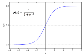
\[f(x) = \frac{e^x}{1 + e^x}\]Let’s see what this function looks like, here it is:

See how it has an S-shape, it is a very useful property of this function. Another very useful property of this function is that the derivative of this function is easily written in terms of the function itself. Specifically:
\[\nabla f(x) = f(x)(1 - f(x))\]So, what does the property of always being in the interval \([0,1]\) mean to us? Well, it means that we can assign labels, or class numbers with the help of a threshold (usually = \(0.5\)). So that if \(y < 0.5\), we assign class 0. Else if \(y >= 0.5\), we assign class 1. But how can we use this function to make predictions by learning from data? We see this below.
Idea Of The Problem
Remember that last time the error function we minimized was the sum-of-squares error function given by:
\[\frac{1}{2}\sum_{n=1}^N (y_n - t_n)^2\]Where \(t_n\) is the label for the n-th training example and \(y_n\) is our prediction for the n-th training example.
In the case of the classification problem, it is easy to see that this function is not descriptive as we would like. As now the labels and our predictions are going to be one of two possible values, either \(0\) or \(1\). So that the terms in the above sum will be either \(0\) or \(1\) (make sure you convince yourself of this). We therefore use a different function to measure the error.
This function is called the cross-entropy error function and is given by:
\[-\sum_{n=1}^N {t_n}\log(y_n) + (1 - t_n)\log(1 - y_n)\]Here the notation is the same as above, except that \(y_n = f(a_n)\), where \(a_n = {w}^T{x_n} + b\) but now \(f\) is the logistic sigmoid function. We derive the cross entropy function below. If you are not instantly comfortable with all the details, don’t worry, the key insight to take is this:
In Machine Learning, it is always a good idea, or rather, an extremely powerful framework, to write the error as the negative of our probability assignment function.
This is because minimizing the negative of something corresponds to maximizing its positive. So that when our error function, so defined, is minimized, our probability function tends to assign high probabilities to correct classes.
Posing The Problem
The problem to solve here is going to an optimization problem, similar to the one in the last post. But we arrive at it through a slighly different route. Namely, through the idea of Maximum Likelihood.
This method looks to maximize the possibility of the occurence of the optimum value of some variable. We call it optimizing the objective function with respect to this variable. Here is the method:
We start by noting that each of our prediction is going to be in one of two classes. So that we can write our probability as:
\[p(x_n) = {y_n}^{t_n} ({1 - y_n}^{1 - t_n})\]where \(t_n\) is either \(0\) or \(1\), \(y_n\) is our prediction. We write down the Likelihood function, this is the product of the above term, just for all \(N\) terms in the dataset:
\[L(X) = \prod_{n=1}^N p(x_n) = \prod_{n=1}^N {y_n}^{t_n} ({1 - y_n}^{1 - t_n})\]Here X denotes the whole dataset consisting of all examples \(x_n\). If we take the negative logarithm of this above equation, and note the three properties shown below:
1. \(log(xy) = log(x) + log(y)\)
2. \(log(e^{x}) = e^{log(x)} = x\)
3. \(a^x = e^{x log(a)}\)
we get:
\[E(w) = -\sum_{n=1}^N {t_n}\log(y_n) + (1 - t_n)\log(1 - y_n)\]Now, if we take the gradient of this function with respect to \(w\) (remember that \(y_n = f(a_n)\), where \(a_n = {w}^T{x_n} + b\)), and rearrange, we get:
\[\nabla E(w) = \sum_{n=1}^N (y_n - t_n)x_n\]This is the function we have to minimize.
Solving The Problem
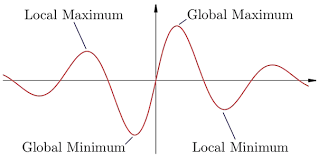
Now, see that our function \(f\) is no longer a linear function, but a non-linear function, given by the logistic sigmoid. The surface of the error function is now like a landscape, with many mountains (local maxima) and valleys (local minima). So, simply setting the above equation to zero won’t give us our answer, we need another approach.

Here, we take an iterative approach, in which we do not solve the whole problem in one shot like we did with plain linear regression, but rather we solve the problem in a finite number of steps. The approach we use is called the Newton-Raphson Method. It has the simple but powerful formulation:
\[w^{new} = w^{old} - {H}^{-1}\nabla E(w)\]Where \(\nabla E(w)\) is the gradient of the error function, which we have derived above. \({H}^{-1}\) is the inverse of the Hessian Matrix. This matrix contains the second derivatives of the error function \(E\) with respect to \(w\), that is, \(H = \nabla \nabla E(w)\).
We are very close to solving this problem, just a few more steps!
We can write \(\nabla E(w)\) in a vectorized form, such as this:
\[\nabla E(w) = {X^T}(y - t)\]Here, we have collected all \(y_n\) and \(t_n\) in the vectors \(y\) and \(t\) respectively. Also, we collected all input vectors \(x_n\) into a single matrix \(X\).
Using this, the last piece required is the Hessian, which can be obtained by differentiating the immediately above equation once more with respect to \(w\) to obtain:
\[H = \nabla\nabla E(w) = \sum_{n=1}^N y_n(1 - y_n){x_n}{x_n}^T = {X^T}RX\]Here, \(R\) is a diagonal matrix (all entries not on the diagonal are zero. Mathematically, \(R_{i, j} = 0\) if \(i \neq j\). Using the property of the derivative of the logistic sigmoid, the diagonal elements of \(R\) are given by:
\[R_{nn} = f_n(1 - f_n)\]where \(f_n\) = \(f(a_n)\)
Finally, the last step just involves putting these terms together in the Newton-Raphson Method, which, recall, was:
\[w^{new} = w^{old} - {H}^{-1} \nabla E(w)\]Substituting into these equations the values we have just derived, we get:
\[w^{new} = w^{old} - ({X^TRX})^{-1}{X^T}(y-t)\]We have to repeat this step some finite number of times. In this case, we replace \(new\) by \(N\), and \(old\) by \(N - 1\). The update steps then become:
\[w^{N} = w^{N - 1} - ({X^TRX})^{-1}{X^T}(y-t)\]And we choose an initial value for \(w^{0}\), say \(w^{0} = 0\), the zero vector.
And that’s it!
Now, we can finally implement this algorithm in code!
Implementing The Algorithm In Code
import numpy as np
import sklearn.datasets
import matplotlib.pyplot as plt


def train(X, y, w_init, n_iterations):
	y_ = prepare_predictions(X, w_init)
	R = np.zeros((X.shape[0], X.shape[0]))
	error_log = []
	for k in range(R.shape[0]):
		R[k][k] = grad_logistic_sigmoid(y_[k])

	H = np.matmul(X.T, np.matmul(R, X))
	w = w_init
	grad_E = np.matmul(X.T, (y_ - y))
	for n in range(n_iterations):
		error = cross_entropy_error(y_, labels)
		error_log.append(error)
		print('error at iteration {} = {}'.format(n + 1, error[0]))
		w = newton_raphson(w, H, grad_E)
		y_ = prepare_predictions(X, w)
		updated_params = update_matrices(X, y_, y)
		grad_E, H, R = updated_params[0], updated_params[1], updated_params[2]

	return w, error_log


def update_matrices(X, y_, y):
	R = np.zeros((X.shape[0], X.shape[0]))
	for k in range(R.shape[0]):
		R[k][k] = grad_logistic_sigmoid(y_[k])
		H = np.matmul(X.T, np.matmul(R, X))
		grad_E = np.matmul(X.T, (y_ - y))
	return grad_E, H, R


def cross_entropy_error(y_, labels):
	error = 0
	for n in range(len(y_)):
		error += (labels[n] * stable_log(y_[n])) + (1 - labels[n]) * stable_log(1 - y_[n])
	return -error


def prepare_predictions(X, w, classify=False):
	y_ = [0 for j in range(X.shape[0])]
	for k in range(X.shape[0]):
		sample = X[k, :]
		sample = sample.reshape(sample.shape[0], 1)
		prediction = predictions(sample, w, classify)
		y_[k] = prediction
	y_ = np.array(y_)
	return y_.reshape(y_.shape[0], 1)


def logistic_sigmoid(x):
	return stable_sigmoid(x)


def grad_logistic_sigmoid(x):
	return logistic_sigmoid(x) * (1 - logistic_sigmoid(x))


def predictions(x, w, classify=False):
	linear_comb = np.matmul(w.T, x)
	pred = logistic_sigmoid(linear_comb)
	if classify:
		if pred >= 0.5:
			pred = 1
		else:
			pred = 0
	return pred


def newton_raphson(w_old, H, grad_E):
	w_new = w_old - np.matmul(np.linalg.inv(H), grad_E)
	return w_new


def stable_sigmoid(x):
    squashed_x = np.zeros(x.shape[0]).reshape(x.shape[0], 1)
    for j in range(len(x)):
        if x[j] >= 0:
            z = np.power(np.e, -x[j])
            squashed_x[j] = 1 / (1 + z)
        else:
            z = np.power(np.e, x[j])
            squashed_x[j] = z / (1 + z)
    return squashed_x


def stable_log(x, delta=1e-10, epsilon=1e10):
	if x >= epsilon:
		return np.log(epsilon)
	if x <= delta:
		return np.log(delta)
	return np.log(x)


dataset = sklearn.datasets.load_breast_cancer()
features = dataset['data']
labels = dataset['target']
labels = labels.reshape(labels.shape[0], 1)

n_iterations = 100
init_array = np.array([0 for j in range(features.shape[1])])
init_array = init_array.reshape(init_array.shape[0], 1)
w_init = init_array
f_train = features[:500]
l_train = labels[:500]
f_test = features[500:]
l_test = labels[500:]
train_algorithm = train(f_train, l_train, w_init, n_iterations)
w_final = train_algorithm[0]
error_log = train_algorithm[1]
error_log = np.array(error_log)

correct = 0
for j in range(f_test.shape[0]):
	sample = f_test[j, :]
	pred = predictions(sample, w_final, classify=True)
	if pred == l_test[j]:
		correct += 1

print('accuracy = {} %'.format((correct / l_test.shape[0]) * 100))

plt.plot(error_log)
plt.ylabel("Error")
plt.xlabel("Iteration")
plt.show()
We have seen a lot of this code before in the previous post. Here we use the stable_log function to keep a lower and an upper bound for the function, so that it does not result in numerical overflow / underflow.
The parameter n_iterations sets how many iterations we want of the method. The function stable_sigmoid also ensures numerical stability.
The function newton_raphson applies the equation we derived before. The function grad_logistic_sigmoid uses the definition for the gradient that we derived. The function prepare_predictions prepares our vector of \(y_n\) for all \(n\) and then combines them all into a single vector \(y\).
The function predictions performs the actual prediction, it is also controlled by a parameter classify that assigns classes if it is set to True.
The function cross_entropy_error calculates the error using the definition for it we derived previously. While the function update_matrices recomputes \(\nabla E, H^{-1}\) and \(R\) for each new value of \(w\). The whole training is initiated with the function train.
Lastly, at the end, we make predictions on the test set, record accuracy, and display error progress over time on a graph.
And this completes Logistic Regression! Congratulations if you made it this far!
In the next post, we will start looking at Deep Learning and Artifical Neural Networks, the buzz of the day. So Stay Tuned! Thanks for Reading and I’ll see you next time!